Feedback Control
Back to se380
What is control engineering?
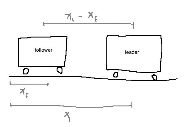
e.g. Automated highway

Objective:
- decide on the velocity commands to the follower in order to maintain a safe inter-vehicle distance
Assumptions:
- cars only move forward and reverse on flat ground
- through software running on an embedded computer, we can assign different velocities to the follower
- Model for follower: \(\frac{df(t)}{dt} = u(t)\), where we decide \(u(t)\)
- Leader moves at a constant but unknown speed
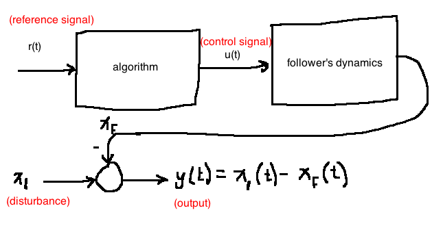
Solution 1: Open loop
- Don't equip follower with any sensors (save that money 💰)
- algorithm to decide velocity only has access to the desired inter-vehicle distance, labelled \(r(t)\)

- Since the algorithm has no access to \(y(t)\), it can't make an informed decision
- Toasters work like this (doesn't sense toast burntness, just goes for a set time)
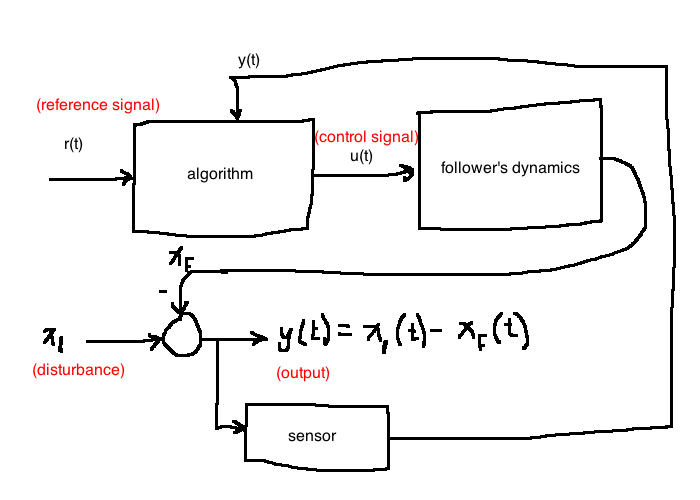
Solution 2: Closed Loop
- equip the follower with sensors that can measure \(y(t)\)

- Simplest control algorithm
- \(u(t) = -K_p (r(t) - y(t)), \quad K_p \gt 0\)
- Better control algorithm: proportional-integral error feedback
- \(u(t) = -K_p (r(t) - y(t)) - K_i \int_0^t{(r(T)-y(T)) dT}, \quad K_p, K_i \gt 0\)
e.g. Web server
(See 1.4.1 in the notes)
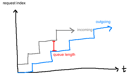
- Web server that responds to GET and POST requests from browsers
- The server has a buffer of pending requests so no requests are lost

Control objectives
- Don't let the queue length get too large (buffer may overflow and requests will be lost)
- Don't let queue length get to zero (it would be a waste of resources to have the server idle)
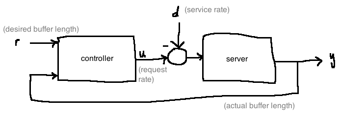
Consequently, we want to keep the queue length at some known value \(r(t)\).
The difficulty is that the service rate is not known, as it depends on many things (e.g. number of clients). Because of this, we will model it as a disturbance \(d(t)\).
We must decide on the request rate \(u(t)\) based on \(r(t)\) and \(y(t)\) (queue length).

Definition
Control engineering attempts to change the behaviour of a system (called a "plant") in a useful way despite the presence of external influences ("disturbances") and despite model uncertainty.
We change the behaviour of the plant by connecting it to another system ("controller"). Feedback is the most powerful interconncetion strategy.
Control Cycle
- Sense the operation of a system
- Compare against a desired behaviour
- Compute a correctibe action informed bu a model of the sustem's respnse to external stimuli
- Actuate the sustem to affect the desired change
The sense, compute, actuate cycle loops.
Design Cycle
- Study the system to be controlled, decide on sensors and actuators. Sensors change what information is at your disposal, and actuators represent choices you can make in response to the inputs.
- Model the resulting system
- mathematical model
- often one or more differential equations, obtained through analysis or experimental data
- Simplify model if necessary
- classical control (this course) deals with linear, time-invariant systems. It requires that we have a transfer function of the plant.
- e.g. \(\mathcal{L}\left\{\frac{dx_f}{dt}\right\} = \mathcal{L}\{u\} \Rightarrow sX_f(s) = U(s)\). Transfer function is \(\frac{X_f(s)}{U(s)} = \frac{1}{s}\).
- A system has a transfer function iff it is linear and time-invariant.
- Analyze the resulting system
- Determine specifications: stability, good steady-state behaviour, robustness, good transient performance
- Decide on type of controller
- Design the controller
- In this course, the controller itself that we design will be a transfer function
- This transfer function corresponds to a differential equation relating the inputs and outputs of the controller
- Simulate (usually using Matlab)
- Return to step 1 if neecessary
- Implement controller
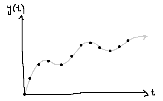
- Realistically, the Ordinary Differential Equation (ODE) from step 7 is discretized and approximated as a difference equation and implemented in software
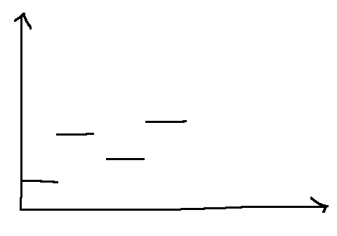
e.g. follower is \(u(t) = -K_p (r(kT)-y(kT)), \quad kT \le t \lt (k+1)T\)
Analog to digital:

Digital to analog:
